Feature importances with forests of trees

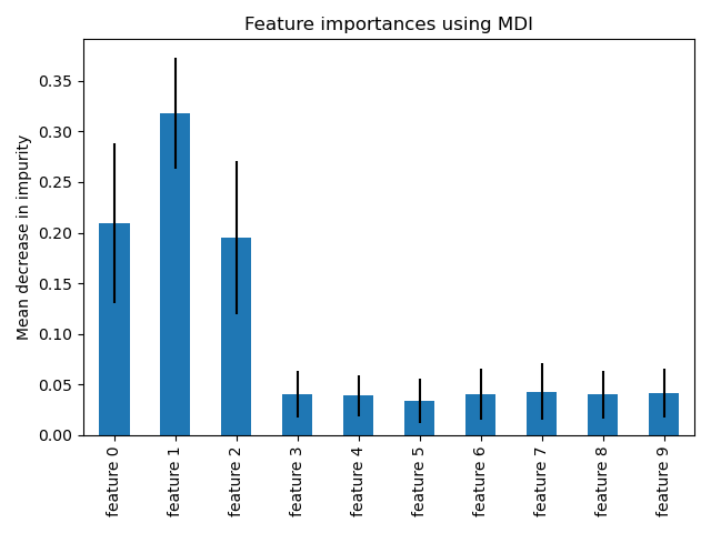
This examples shows the use of forests of trees to evaluate the importance of features on an artificial classification task. The red bars are the feature importances of the forest, along with their inter-trees variability.

As expected, the plot suggests that 3 features are informative, while the remaining are not.

Out:

  Feature ranking:
1. feature 2 (0.426095)
2. feature 1 (0.231205)
3. feature 0 (0.119869)
4. feature 7 (0.033903)
5. feature 9 (0.032583)
6. feature 5 (0.032281)
7. feature 3 (0.032158)
8. feature 4 (0.031123)
9. feature 8 (0.030538)
10. feature 6 (0.030246)

print(__doc__)

import numpy as np
import matplotlib.pyplot as plt

from sklearn.datasets import make_classification
from sklearn.ensemble import ExtraTreesClassifier

# Build a classification task using 3 informative features
X, y = make_classification(n_samples=1000,
                           n_features=10,
                           n_informative=3,
                           n_redundant=0,
                           n_repeated=0,
                           n_classes=2,
                           random_state=0,
                           shuffle=False)

# Build a forest and compute the feature importances
forest = ExtraTreesClassifier(n_estimators=250,
                              random_state=0)

forest.fit(X, y)
importances = forest.feature_importances_
std = np.std([tree.feature_importances_ for tree in forest.estimators_],
             axis=0)
indices = np.argsort(importances)[::-1]

# Print the feature ranking
print("Feature ranking:")

for f in range(X.shape[1]):
    print("%d. feature %d (%f)" % (f + 1, indices[f], importances[indices[f]]))

# Plot the feature importances of the forest
plt.figure()
plt.title("Feature importances")
plt.bar(range(X.shape[1]), importances[indices],
       color="r", yerr=std[indices], align="center")
plt.xticks(range(X.shape[1]), indices)
plt.xlim([-1, X.shape[1]])
plt.show()

Total running time of the script: (0 minutes 1.186 seconds)